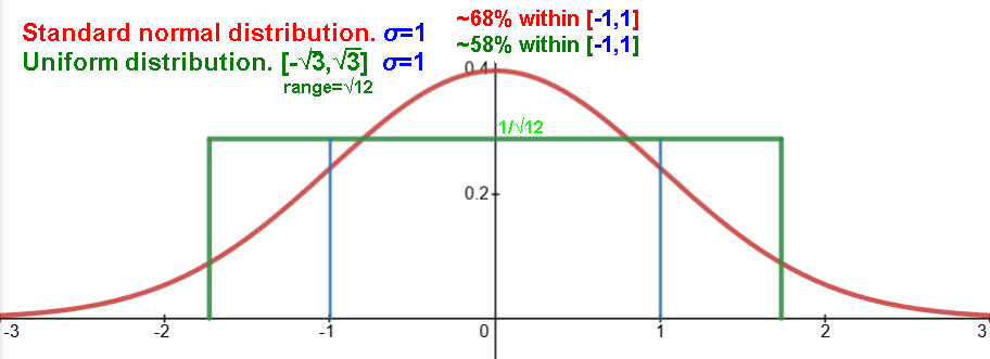
Uniform distribution: every value in range [a,b] equally likely.
mean=(a+b)/2 ie. =midrange=median
standard deviation SD = (b-a)/√12 ≈ (b-a)/3.464
~57.75% of data within 1 SD of mean, all is within 2 SD of mean.
MAD=range/4 Avg.diff.pair=range/3 ?
skew: 0
CDF(x)=P[X≤x]= (x-a)/(b-a)
Quantile InverseCDF Q(p)= p(b-a)+a =x
Normal/Gaussian distribution: quantity that is the sum of many small independent processes.
Also, distribution of samples' means.
mean=median=mode
~68% of data within 1 SD of mean, 95%..2 SD.., 99.7%..3 SD..
MAD=σ√(2/π)=.7979σ Avg.diff.pair=2σ/√π≈1.128σ
skew: 0
kurtosis: 0
Generate correlated normal data
Binomial distribution: #successes/yeses/ones in n tries when probability of a success is p.
mean= np
standard deviation= √(np(1-p))
skew: (1-2p)/σ
kurtosis: (1-6p(1-p))/σ2
n=1 : Bernoulli distribution. p=proportion success
Poisson distribution: λ=expected/average independent #events in an interval.
Probabilities of each k (0-) #occurences/events/arrivals in an interval.
mean= λ
standard deviation= √λ
skew: 1/√λ
kurtosis: 1/√λ
Χ2 Chi-squared distribution: sum of k squared standard normals
mean= k
standard deviation= √(2k)
skew:√(8/k)
kurtosis: 12/k ?
Lognormal distribution: its log is normally distributed.
μ and σ are mean and standard deviation of that normal distribution.
mean= eμ+σ2/2
mode= eμ-σ2
median= eμ
mode<median<mean
standard deviation= eμ+σ2/2√(eσ2-1)
Exponential distribution: λ=rate of happening = 1/avg.wait time
mean= 1/λ
median= μ ln 2 <μ
standard deviation= 1/λ
~95.02% of data within 2 SD of mean.
pdf= λe-λx
CDF(x)=P[X≤x]= 1-e-λx
Quantile InverseCDF Q(p)= -ln(1-p) / λ
t distribution: ν=degrees of freedom
mean=0
σ=√(ν/(ν-2)) ν>2
skew= 0 ν>4, undefined 1,2,3
kurtosis= 6/(ν-4) ν>4, ∞ 3,4, undefined 1,2
