applied to categorical data to evaluate how likely it is
that differences between the actual observed data
and its expected/theoretical values arose by chance.
It tests a null hypothesis that the frequency distribution of certain
events observed in a sample is consistent with a particular theoretical distribution.
The events must be mutually exclusive and have total probability 1.
video. die 30 rolls:
#1s #2s #3s #4s #5s #6s
 3   3   4   8   7   5
Expected uniform distro: 1/6*30
 5   5   5   5   5   5

book: 45 die rolls:
13   6  12   9   3  2
Expected uniform distro: 1/6*45
7.5 7.5 7.5 7.5 7.5 7.5

book: loaded die 45 rolls
13    6   12   9   3  2
22.5 4.5 4.5 4.5 4.5 4.5

last digit of self-reported weights  n=2784
1175 44 169 111 112 731 96 110 171 65
every E= 1/10*2784= 278.4  Expected uniform distro

Benford's law E
.301 .176 .125 .097 .079 .067 .058 .051 .046

Leading digits packet interarrival time
69 40 42 26 25 16 16 17 20    =271
271*Ei:
81.571 47.696 33.875 26.287 21.409 18.157 15.718 13.821 12.466

76 62 29 33 19 27 28 21 22
95.417 55.792 39.625 30.749 25.043 21.239 18.386 16.167 14.582


V-1
229 211 93 35 8
227.5 211.4 97.9 30.5 8.7

Kentucky Derby
19 14 11 15 16 7 9 12 5 11   =119
every E=119/10= 11.9

Old Faithful.  classwidth 10. Drop outlier 125   n=49
2 0 3 9 23 10 2
hmm, won't work on tails? <5
0.0029 0.0259 0.1165 0.2690 0.3191 0.1947 0.0610

The day-of-birth data in Nominal Data
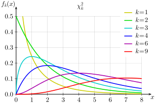
PDFs of chi-squared functions for first few values of k:
Sum of k squared random selections from the standard normal distribution.
Expected value of Χ2k = k
Variance of Χ2k = 2k
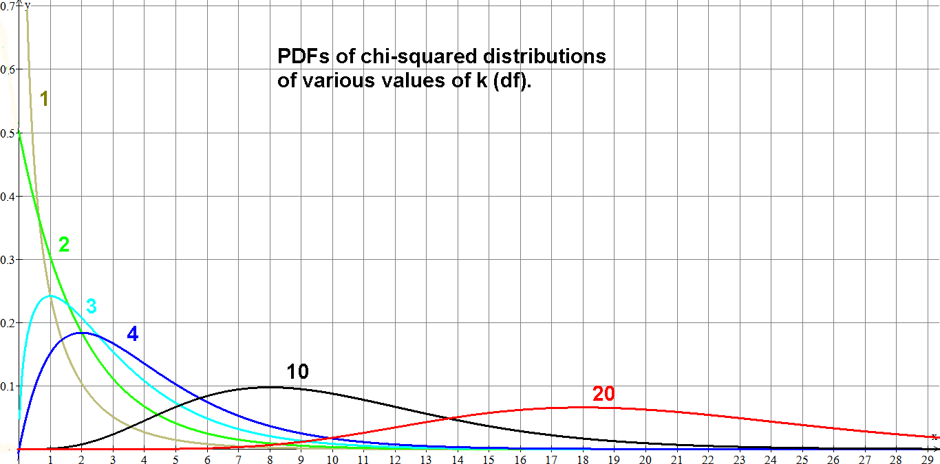
PDFs of chi-squared functions for various values of k:
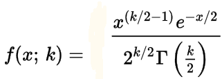 Γ gamma function
| k | Γ(k/2) | =/≈ |
|---|---|---|
| 1 | Γ(1/2) | 1.7724 |
| 2 | Γ(1) | 1 |
| 3 | Γ(3/2) | .8862 |
| 4 | Γ(2)=1! | 1 |
| 5 | Γ(5/2) | 1.3293 |
| 6 | Γ(3)=2! | 2 |
| 7 | Γ(7/2) | 3.3233 |
| 8 | Γ(4)=3! | 6 |
| 9 | Γ(9/2) | |
| 10 | Γ(5)=4! | 24 |
| 20 | Γ(10)9! | 362880 |
Mathpapa k= 1, 2, 3
y=\frac{x^{\left(\frac{1}{2}-1\right)}e^{-\frac{x}{2}}}{2^{\frac{1}{2}}\cdot 1.7724}\ \ ;\ \ \ \ y=\frac{x^{\left(\frac{2}{2}-1\right)}e^{-\frac{x}{2}}}{2^{\frac{2}{2}}}\ ;y=\frac{x^{\left(\frac{3}{2}-1\right)}e^{-\frac{x}{2}}}{2^{\frac{3}{2}}\cdot .8862}