Standard deviation SD

Measures the spread of the data around the mean, i.e. its variation.
An average of how much the data deviates from or around the mean.
A measure of how much we can expect a value to differ from the center.
A measure of the uncertainty there is for any data value.
The more spread out, the more dispersed, the more scattered the data, the larger its standard deviation.
The larger the standard deviation is, the more spread out and dispersed the data.
The more clustered and huddled the data around the mean, the smaller its standard deviation.
SD is never negative; it's either positive or 0.
It has the same unit of measurement as the data.
The most important statistic: it measures the variation, the uncertainty, of the data and it (or its square, the variance) plays a role in many statistical tests.
Invented 1890s by Pearson.

Definition and formula for the standard deviation:

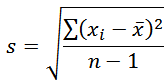
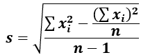
s is the sample standard deviation.
The x_i are the data values, x̄ is the sample mean, n is the number of data values, i.e. the sample size.
Take the difference between each data value and the mean (this differences is the datum's deviation), square that and sum those squared differences (this is the "sum of squares", SS), divide by n-1 for a kind of average squared difference, and then take the square root of that quotient.
Squaring makes it all positive numbers. And gives more "weight" to datums far from the mean.
The square rooting un-does the squarings and gets back the original un-squared units of the data [m, kg, ft, Cal, W, etc.].

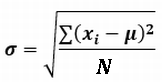
σ (sigma) is the population standard deviation. Uses the population mean μ and divides by N, the population size.
s is always larger than σ but not by much except for small n and N.

NB. Sometimes, someplaces s is denoted by σ_n-1 and σ by σ_n

Webpage to calculate statistics, including standard deviations.

In the sample SD formula, the n-1 is Bessel's correction; it gives slightly better value for small sample sizes n (for large n, eg. 100, there is little difference between dividing by 100 and 99).
The variation in a sample can be no more than that in the population, and is likely to be less. The sum of squared differences is likely to be smaller than the population's, so dividing by the smaller n-1 yields a slightly larger quotient, partially compensating.

Alternate "computational" formula for s. Note it doesn't need the mean.

Exs.:
This data: 1 2 3 4 5 6 7 8 9 10   has a mean of 5.5 and a standard deviation of 2.87.
This data: 0 2 3 4 5 6 7 8 9 11   same mean of 5.5 but a wider spread, and so its standard deviation is larger, at 3.20.
This data: 1 2 3 5 5 5 7 8 9 10   mean of 5.5 but is more "clustered", and its standard deviation is 2.83.
This data: 2 2 3 5 5 5 7 8 9 9    is more clustered yet, and so its standard deviation is 2.53.
The standard deviation is not directly related to the range. This data: 2 4 4 5 5 5 5 6 6 14   has the largest range of these examples but not the largest standard deviation (its is 3.00).
Nor is it related directly to the number of different data values. This data: 1 1 1 5 5 5 5 10 10 10   has the fewest number of different data values but a large standard deviation of 3.49.

If the data is all the same, the standard deviation is zero. There is no variation among the data, it is all [clustered] at the mean. (This is the only way for the SD to be 0.)
Ex.: This data: 5 5 5 5 5 5 5 5 5 5 has SD = 0

For a given range, if the data is perfectly bi-modal, i.e. half is the min and half is the max, then σ is the midrange (i.e. one half the range), which is the distance from the mean to either datum.
Ex.: This data: 10 10 10 10 10 20 20 20 20 20 has mean=15, σ = 5

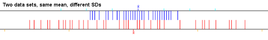
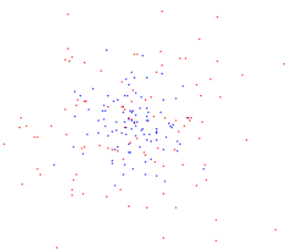
Ex.: The red and blue dots have the same average (at the center of the image) but different standard deviations (red data's SD is larger than the blue data's SD):

Without knowledge of the standard deviation, the mean is incomplete. Standard deviation complements the mean; shouldn't have one without the other.
These data sets have the same mean and the same range:
1 1 1 1 1 9 9 9 9 9 9
1 5 5 5 5 5 5 5 5 9 9
but you wouldn't want to leave it at that. SD will help characterize their differences. SD of the first is 3.98, the second 2.06.

There isn't a perfect geometric/physical idea of what the standard deviation is. It is a kind of average distance of data from the mean.
Mean absolute deviation, MAD, is the average distance from the mean:
MAD
Σ|x_i-x̄| / n    i.e. sum all the distances, divide by the number of them.
MAD≤σ
Exs. SD and MAD



If the data is perfectly bi-modal, σ is one half the range, which is the distance from the mean to either datum, which is the mean [absolute] deviation (MAD). Otherwise, σ > MAD [except if data all same: SD=MAD=0]
Ex.: This data: 10 10 10 10 10 20 20 20 20 20 has σ = 5 = MAD
Unfortunately, the intuitive MAD plays almost no role in stats! The SD is used instead, for theoretical math reasons. SD ≥ MAD. In a normal distribution: SD≈1.25MAD. Uniform distro: SD≈1.73MAD. Exponential distro: SD≈e·MAD
In a normal distribution:

Range rule of thumb: SD is approximately range/4. Can be used to guesstimate SD if no software available etc.

Root mean square (RMS) of a set of values is the square root of the mean of the squares of the data: .
SD of a set of values is the square root of the mean of the squares of the differences of the data and the mean. The "root mean squared difference [or deviation]".
RMS measures average magnitude relative to zero.
SD measures average magnitude relative to the mean.

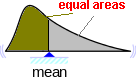
The mean is a balance point, the sum of the distances to the data less than the mean equals the sum of the distances to the data greater than the mean.

Also, the mean splits the histogram/curve into two equal-sized halves, each containing 50% of the area and probability.

The standard deviation is a "natural" measure of dispersion when the "center"/"middle" of the data is the mean, because the standard deviation from the mean is smaller than from any other point, i.e. it is minimized when calculated, as it is, from the mean. It would be larger if any other point were used in the formula.

1 2 3 4 5 6 7 8 9 10 has SD=2.87
Adding the same constant c to each data value does not change the SD.
Add c=100 to each of those numbers gives 101 102 103 104 105 106 107 108 109 110 whose SD is 2.87
Multiplying all the data values by a constant k multiplies the SD by the same number.
Multiplying each of those numbers by k=10 gives 10 20 30 40 50 60 70 80 90 100 whose SD is 28.7
Doubling is multiplying by 2. SD doubles.
Halving is multiplying by 1/2. SD halves.
Increasing/decreasing by p% is multiplying by 1±(p/100)
Duplicating etc. every datum has no effect on the SD.

Coefficient of variation:
sample CV = s / x̄     or population CV = σ / μ
Expressed as a percentage. Basically, is the percent that the SD is of the mean.
How much the data varies compared to the mean. A measure of the spread of the data relative to the average of the data. Useful for comparing data sets whose means are very different or use different measuring units.

Variance
The variance, VAR, is the square of the standard deviation.
Population VAR = σ². Sample VAR = s².
The standard deviation is the square root of the variance: SD = √VAR
Different equivalent formulae for VAR:

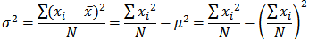
(sample variance has n-1 in place of N).
In the SD formula, if the square root is not done we are left with the VAR.
Variance is more difficult to think about than SD because it is squared and its unit of measurement is unnatural as squared (squared liters, squared Calories, squared °C etc.).
Different fields/disciplines/individuals prefer VAR or SD.
"Variance" is both this statistic/parameter and a synonym for dispersion/spread/uncertainty etc.

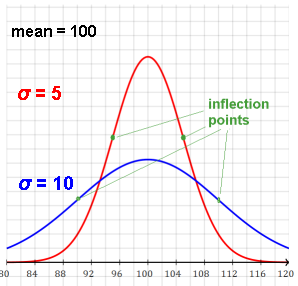
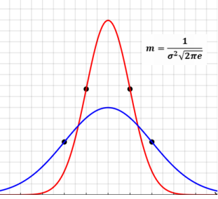
A normal/Gaussian probability distribution/density function (PDF) is characterized/defined by its mean μ and σ.

Here are the graphs of three normal distribution functions with the same mean of 10 but different standard deviations of 1, 2, and 3:
u=10, blue s=1, red s=2, green s=3

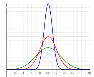
The area under the curve of each function is the same, i.e. 1.
The smaller the σ, the narrower and taller the curve, the more clustered around the mean.
The larger the σ, the wider and shorter the curve, the more dispersed around the mean.

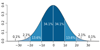
Empirical Rule of a Normal Distribution:
~68% of data within 1 σ of mean,
~95% of data within 2 σ,
~99.7% of data within 3 σ

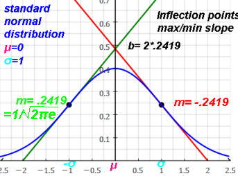
One σ from the mean of a normal curve/function is an inflection point, where the concavity changes sign, where the second derivative is zero, where the slope (rate of change) is at a maximum or a negative minimum.
     

Probability Distribution function	Standard deviation	MAD
Uniform	range/√12	range/4
Normal	σ	σ√(2/π)
Binomial	√(np(1-p))
Poisson	√λ
Χ2	√(2k)
Exponential	1/λ
t	√(df/(df-2)), df>2
Lognormal	eμ+σ2/2√(eσ2-1)

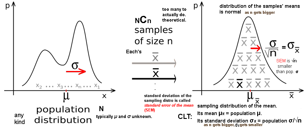
Central Limit Theorem: