CLT central limit theorem demo

Paste the usually unknown
population data:
(Data distribution generator can make any amount of data from various distributions)
      N=
      μ=
      σ=

sample size n:       √n=
#samples:


The sampling distribution of the mean:
Sample means i

Paste into Statistics, frequency distribution, histogram to see its histogram etc.

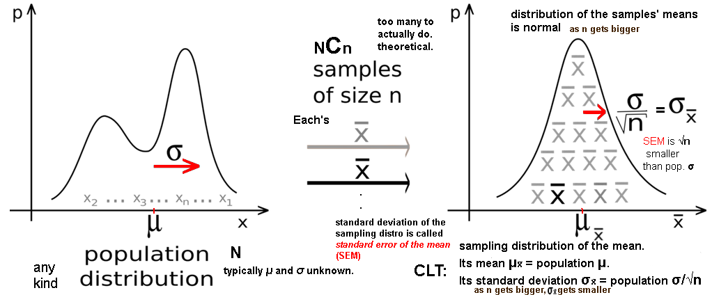
Mean of the sample means μ= ∑x̄i/#samples:   will approach the population μ.

Standard deviation of the sample means (AKA standard error SE, [of the mean] SEM) σ=   will approach the population σ/√n.
    σ·√n= σ

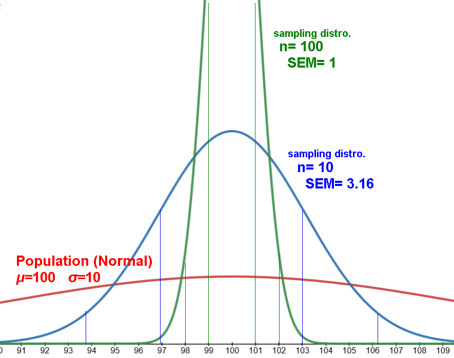
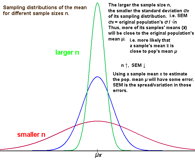
*** A smaller SEM indicates an x̄ is a more precise estimate. better, more reliable, higher "quality". because more/most samples' x̄ will be closer to μ.

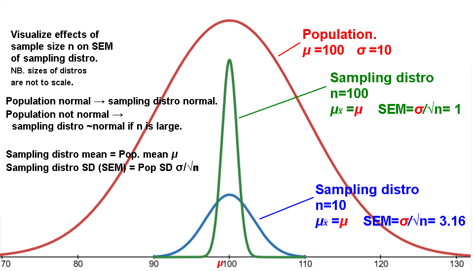
** The mean μ of the sampling distribution of x̄ is equal to the population mean μ [even if the sample size n is small].
** The standard deviation (i.e. SEM) of the sampling distribution of x̄ is equal to σ/√n [even if the population is not normal and even if n is small].
** If the population is normal, the sampling distribution of x̄ is normal, [even if n is small].
*** If n is large, the sampling distribution of x̄ is approximately normal [even if the population is not normal].   ~30 is large enough (except some every non-normal need larger n)
CLT does not apply if the observations are not independent, e.g. without replacement.

*** In real life we almost never know σ. 
So we replace it with the sample standard deviation s and compute the estimated standard error = s/√n.
s is a consistent estimator of σ: as n increases, s gets closer to σ, so s/√n gets closer to the true SEM.

For smaller samples the substitution introduces extra uncertainty, 
 which is why we switch from the normal (z) distribution to the t-distribution 
 when we build confidence intervals (t-Interval) or perform hypothesis t-tests. 
The heavier tails of the t-distribution compensate for the fact that we had to estimate σ rather than knowing it.
s is used in place of σ because it is the best estimate of the population standard deviation that the sample gives us. 
The t-procedures then properly account for the additional uncertainty that comes from that estimation.

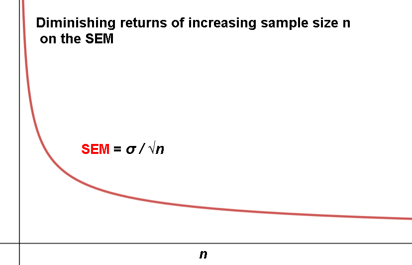
As n increases, the SEM decreases as the root of n:

n σ cf. σ
4 1/2
16 1/4
64 1/8
256 1/16
Quadruple the sample size n to halve the σ.

The sampling distribution of the standard deviation:
Sample standard deviations si

Paste into Statistics, frequency distribution, histogram to see its histogram etc.

Mean of the sample standard deviations =∑si/#samples:


The sampling distribution of the proportion p̂.

Mean equal to population proportion p.
Standard deviation equal to √[p(1-p)/n]
   which is approximately normal provided that np and n(1-p) are large enough (5 or 10).


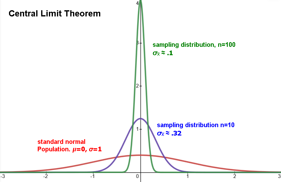
Standard normal pop. μ=0. σ=1  N=100,000
10,000 samples of n=10 --> σ≈ .32
10,000 samples of n=100 --> σ≈ .1

Uniform pop. [0,100]  μ=50. σ=29  N=100,000
10,000 samples of n=10 --> σ≈ 9.2  range~20-80
10,000 samples of n=100 --> σ≈ 2.9 range~40-60

Exponential pop. λ=.1  μ=10. σ=10  N=100,000
10,000 samples of n=10 --> σ≈ 3.16  range~2-27
10,000 samples of n=100 --> σ≈ 1 range~7-14