Data distributions: Uniform, Normal, Skewed, Bimodal
| Uniform
| Normal
| Right-skewed
|
| 
| 
|

| 
| 
|
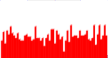
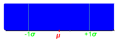
quartiles all same length
mean≈median
no mode
no outliers
SD≈range/√12 = range/2/√3
~58% of data within 1 SD of mean,
all data within ~√3 SD
| 1st Q≈4th Q 2nd Q≈3rd Q
1,4th Qs longer than 2,3rd Qs
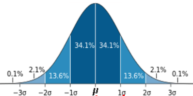
mean≈median≈mode (modal class)
outliers
~68% of data within 1 SD of mean,
~95% within 2 SD,
~99.7% within 3 SD
| quartiles increase in length
(1Q<2Q<3Q<4Q)
median < mean
outliers on right
|
| 
|
|
Normal Data
Very Strong / Textbook Examples

Human heights (adult men or women within one population group)
Adult male heights in the US: mean ~175 cm, SD ~7 cm
Adult female heights: mean ~162 cm, SD ~6–7 cm
Very close to normal when measured in large samples from a single ethnic/geographic group.

IQ scores (standardized tests like WAIS, Stanford-Binet)
Designed to be normally distributed: mean = 100, SD = 15 (by construction).
One of the purest real-world normal distributions.

Birth weights (full-term infants in a population)
Mean ~3.4 kg, SD ~0.5 kg
Very close to normal for healthy, full-term babies.

Measurement errors (in repeated measurements of the same object)
Length of a metal rod measured 50 times with a caliper
Errors due to small random fluctuations → almost perfectly normal.

Blood pressure (systolic or diastolic in a healthy adult population)
Systolic BP in adults: often close to normal (mean ~120 mmHg, SD ~15–20 mmHg) when excluding hypertension cases.


Examples That Are Approximately Normal (Good Enough in Practice)

Test scores on standardized exams (SAT, ACT, GRE, etc.)
Scores are deliberately scaled to be roughly normal (mean 500–1000 range, SD ~100–200 depending on test).

Body mass index (BMI) in large adult populations
When excluding extremes (severe obesity or underweight), BMI often looks roughly normal.

Reaction times (simple visual or auditory reaction time tasks)
In controlled lab settings, reaction times are close to normal after removing outliers.

Residuals in regression models
In linear regression, the residuals (errors) are often assumed and observed to be
 normally distributed when the model fits well.
Right-skewed data:
  Income / wealth distributions
  Time to failure of mechanical parts (exponential)
  Time between customer arrivals (exponential inter-arrival)
  Insurance claim sizes
  Sizes of cities / populations
  Sizes of earthquakes (Richter scale)
  Sizes of forest fires / natural disasters
  Number of children per family
  Time spent on websites / app sessions
  Number of social media followers / likes
  Sizes of companies (employees, revenue)
  Word lengths in texts
  Sizes of file downloads / internet traffic
  Bacterial colony counts
  Particle sizes in aerosols or sediments
  Waiting times in queues
Uniform

Discrete:
 dice   coins   cards   lottery  random digit
Continuous:
  Waiting time for event that occurs exactly every T time_units (random arrival),  [0,T]
  Spinner  angle, [0° to 360°)
  Quantization error in analog-to-digital conversion (ADC),  [–½ LSB, +½ LSB]
  Random arrival time within a fixed interval,  e.g. [0,60]
  Idealized random number generator (RNG),  [0,1)
  Position of a raindrop on a short, straight line segment (idealized).
  Certain manufacturing tolerances when a process is tightly controlled and has no preferred value inside the tolerance band.
  Random selection of a point on a line segment or in a simple geometric region (in pure mathematical models).
True continuous uniform data are relatively uncommon in nature.

Pure uniform distributions are more common in designed systems (dice, lotteries, random-number generators, ideal waiting-time models)
 than in uncontrolled natural phenomena.


Bimodal
A sample that looks clearly bimodal (two distinct peaks) is frequently the result of mixing data
 from two different populations or processes.
 This is the most common and natural explanation.
Typical cases where it really is two populations:
  Male and female heights or weights (when the means are far enough apart)
  Two different machines, shifts, or operators producing measurements
  Two distinct groups in a study (e.g., treated vs untreated, two species, two age cohorts)
  Before-and-after data accidentally combined
In these situations the observed distribution is a mixture of two underlying distributions.

Other causes can produce a bimodal appearance:
  Natural single-population bimodality: Some traits are inherently bimodal
   (certain animal sizes, age of onset of some diseases, etc.)
  Sampling or binning artifacts: Histogram bin width or small sample size can create the illusion of two peaks
  Threshold or nonlinear effects: A process with a sharp threshold can turn a unimodal input into a bimodal output
  Mixture of more than two groups Or unequal variances that create a shoulder that looks like a second mode
  Measurement issues: Two different instruments or methods combined

Practical rule of thumb
  Clear, well-separated peaks → strong suggestion of two (or more) underlying groups.
    Investigate by splitting the data (e.g., by sex, machine, batch, etc.).
  Mild or ambiguous bimodality → be more cautious; it may be noise, binning, or a single skewed distribution.

Bottom line:
  A bimodal-looking sample probably comes from two populations or processes,
   and that is the first hypothesis worth checking.
  It is not automatic proof, however — always look for a substantive reason for
   the two peaks rather than assuming mixture solely from the shape of the histogram.