See whether a frequency distribution fits, or conforms to, a particular distribution (a specific pattern).
Applied to categorical data to evaluate how likely it is
that differences between the actual observed data
and its expected/theoretical values arose by chance.
It tests a null hypothesis H0 that the frequency distribution of certain
events observed in a sample is consistent with a particular theoretical distribution.
I.e. the observed distribution does not differ significantly from the expected distribution.
H0: good fit between Observed and Expected(Theoretical).
HA: not a good fit between Observed and Expected(Theoretical).
So actually testing for badness of fit.
Is what is observed too far away from what is expected, given random fluctuations?
The events must be mutually exclusive and have total probability 1.
Are the differences between the sample's frequencies and the theoretical frequencies significant?
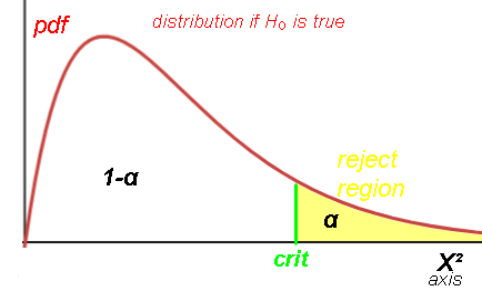
(if so, reject H0).
Or are the differences just due to random chance? (so fail to reject H0).
Excel: Line chart w/marker
category Oi Ei
video. die 30 rolls:
#1s #2s #3s #4s #5s #6s
 3   3   4   8   7   5
Expected uniform distro: 1/6*30
 5   5   5   5   5   5

Try: Oi
 1   3   4   8   9  5
 1   3   3   9   9  5


book: 45 die rolls:
13   6  12   9   3  2
Expected uniform distro: 1/6*45
7.5 7.5 7.5 7.5 7.5 7.5

DataMListic: 60 rolls
 7  9  8 11  6 19
10 10 10 10 10 10

book: loaded die 45 rolls. 1 50%, 2-6 10%
13    6   12   9   3  2
22.5 4.5 4.5 4.5 4.5 4.5


*2 dice sum
      2         3       4      5        6      7           8        9      10       11     12
E= .027777  .055555  .083333 .111111 .1388888 .16666666 .1388888 .111111 .083333 .055555 .027777
n=100
Ei= 2.7777 5.5555 8.3333 11.1111 13.88888 16.666666 13.88888 11.1111 8.3333 5.5555 2.7777
Oi= 2       5      6     17      12       16        13        9      13      7      0
Oi= 5       3      7     17       9       11        10       12      14      7      5
Oi= 6       3      7     17       9       10         9       12      14      7      6


last digit of self-reported weights  n=2784
1175 44 169 111 112 731 96 110 171 65
every E= 1/10*2784= 278.4  Expected uniform distro


Benford's law   Leading digit:
     1    2    3    4    5    6    7    8    9
Pi= .301 .176 .125 .097 .079 .067 .058 .051 .046

Leading digit of packet interarrival time
69     40     42     26     25     16     16     17     20    =271
Ei=271*Pi:
81.571 47.696 33.875 26.287 21.409 18.157 15.718 13.821 12.466

76     62     29     33     19     27     28     21     22    =317
Ei=317*Pi:
95.417 55.792 39.625 30.749 25.043 21.239 18.386 16.167 14.582


V-1 hits. #of the 576 London regions with 0,1,2,3,4 hits of 535 hits
229    211  93   35   8
227.5 211.4 97.9 30.5 8.7     expected Poisson u=.929

*Kentucky Derby
19 14 11 15 16 7 9 12 5 11   =119
every E=119/10= 11.9

19 16 15 15 16 7 9 8 5 7     =119     Changed a bit...


Old Faithful.  classwidth 10. Drop outlier 125   n=49
2 0 3 9 23 10 2
hmm, won't work on tails? <5   "can be combined with another class"
0.0029 0.0259 0.1165 0.2690 0.3191 0.1947 0.0610

Skittles colors   233 "of 4 bags"
Oi:   43 50 44 44 52
Ei:   46.6 46.6 46.6 46.6 46.6

*The day-of-birth data in Nominal Data
57 52 43 53 57 66 72
n=400, each day equally likely, so Ei =400/7= 57.14

Mendel's 556 pea seeds
% smooth-yellow smooth-green wrinkled-yellow wrinkled-green
Oi:  0.5666 0.1942 0.1816 0.0556
Ei:  0.5625 0.1875 0.1875 0.0625
*556:
315.0 108.0 101.0 30.9
312.7 104.2 104.2 34.8
Fisher said : BS, too good to be true

*MLB birthdates months Jan-Dec:    4515
387    329    366    344    336    313    313    503    421    434    398    371
376.25 376.25 376.25 376.25 376.25 376.25 376.25 376.25 376.25 376.25 376.25 376.25
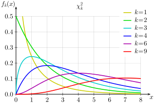
PDFs of chi-squared functions for first few values of df (k):
Area under each curve is 1 (is a probability distro). Small df: right-skewed; large df: becomes symmetric and bell-shaped.
df=1,2: peak at 0. df≥3: peak at df-2.
Sum of k squared random selections from the standard normal distribution.
Expected value of Χ2k = k
Variance of Χ2k = 2k
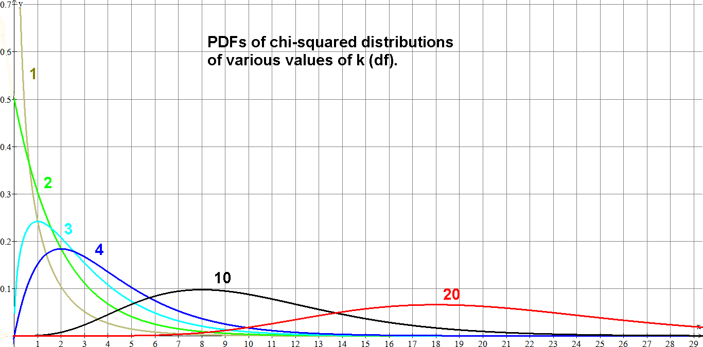
PDFs of chi-squared functions for various values of k:
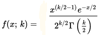 Γ gamma function
| k | Γ(k/2) | =/≈ |
|---|---|---|
| 1 | Γ(1/2) | 1.7724 |
| 2 | Γ(1) | 1 |
| 3 | Γ(3/2) | .8862 |
| 4 | Γ(2)=1! | 1 |
| 5 | Γ(5/2) | 1.3293 |
| 6 | Γ(3)=2! | 2 |
| 7 | Γ(7/2) | 3.3233 |
| 8 | Γ(4)=3! | 6 |
| 9 | Γ(9/2) | |
| 10 | Γ(5)=4! | 24 |
| 20 | Γ(10)9! | 362880 |
Mathpapa k= 1, 2, 3
y=\frac{x^{\left(\frac{1}{2}-1\right)}e^{-\frac{x}{2}}}{2^{\frac{1}{2}}\cdot 1.7724}\ \ ;\ \ \ \ y=\frac{x^{\left(\frac{2}{2}-1\right)}e^{-\frac{x}{2}}}{2^{\frac{2}{2}}}\ ;y=\frac{x^{\left(\frac{3}{2}-1\right)}e^{-\frac{x}{2}}}{2^{\frac{3}{2}}\cdot .8862}