Confidence intervals

One Sample Interval for the Mean μ (t-Interval, t-based confidence interval)

Confidence interval for a population mean μ: if do not know σ (this is usually the case).
CI: a range of believable/plausible values for μ based on our sample.
x̄ is a point estimate of μ; we also want an interval estimate of it.

Underlying machinery: the sampling distribution of x̄, the (estimated) standard error of the mean (SEM)≈ s/√n, the t distribution.

Assumes population is Normal or sample size n>30.
Sample must be SRS random.

sample size n:
sample mean x̄:
sample standard deviation s:
Confidence intervals for various confidence levels (90%, 95%, 98%, and 99%) will be calculated.

   

Estimated standard error of the mean (SEM)= s/√n:        df=n-1:degrees of freedom

Margin of error, E = t critical value * standard error

maximum amount of error by which x̄ misses μ

t_c = t_α/2    α=1-CL    t_c depends on n and CL. (look at T table)

      Confidence interval is x̄±E   =   [x̄-E,x̄+E]

Taking a SRS sample of size n, we can be CL% "confident^*" that the confidence interval x̄±E   [x̄-E,x̄+E]   does contain the true mean μ.
MSL: "CL% confident^* that the limits ... actually do contain the value of the population mean μ."
^*"confident" that this procedure will give us confidence intervals containing μ CL% of the times we do the procedure.
NO: CL% chance/probability that μ is in [x̄-E,x̄+E]. Too loose, too informal. but in practice...?
NO no no: CL% of population's data or datums are x̄±E. Totally wrong.
Yes: If we take many samples of this size and make a CI for each, CL% of them will contain the population μ in the CI.

The confidence level (e.g. 95%) does not measure how good or reliable this particular 
 sample mean x̄ is as an estimate of μ.
Confidence level is a property of the method, not of any single sample:
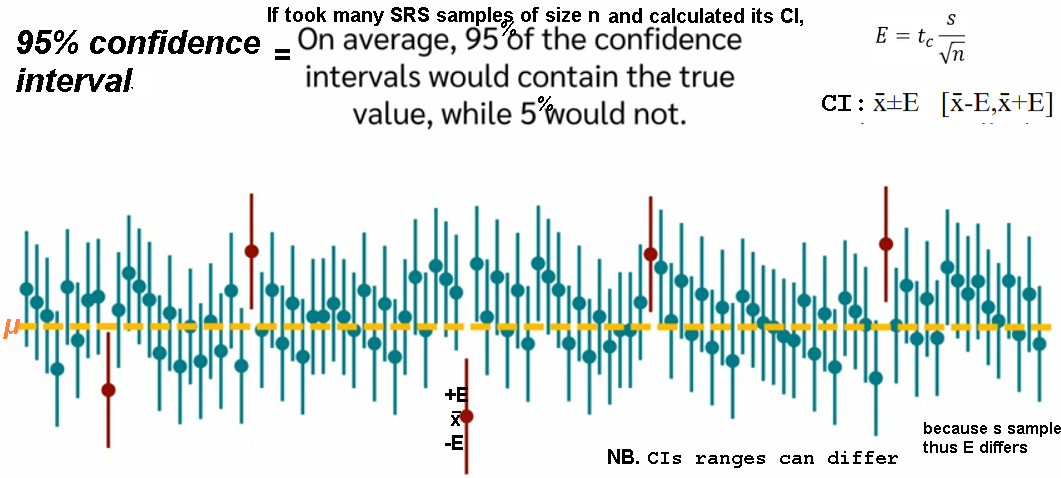
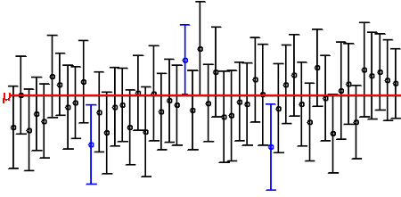
 If we repeated the entire sampling process many times and constructed a 
  confidence interval the same way each time, 
  approximately 95% of those intervals would contain the true population mean μ.
For any one interval that you have in hand, the true μ is either inside it or it isn’t 
 — there is no probability left. 
The “95%” refers to the long-run success rate of the procedure.

A higher confidence level does NOT mean “this x̄ is more trustworthy.”
It makes the interval wider (more cautious), not because x̄ suddenly became better, 
 but because you are demanding a higher long-run capture rate.

Confidence level = reliability of the interval procedure over many repetitions.

*** In real life we almost never know the population standard deviation σ. 
So we replace it with the sample standard deviation s and compute the estimated standard error = s/√n.
s is a consistent estimator of σ: as n increases, s gets closer to σ, so s/√n gets closer to the true SEM.

For smaller samples the substitution introduces extra uncertainty, 
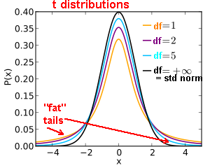
 which is why we switch from the normal (z) distribution to the t-distribution 
 when we build confidence intervals (t-Interval) or perform hypothesis t-tests. 
The heavier tails of the t-distribution compensate for the fact that we had to estimate σ rather than knowing it.
s is used in place of σ because it is the best estimate of the population standard deviation that the sample gives us. 
The t-procedures then properly account for the additional uncertainty that comes from that estimation.

Worksheet

Try: 
36 100 15  At 95% CL E is ~5    At 99% CL E is ~6.8

100 100 10  vs. 1000 100 10   effect of sample size n
100 0 1  vs 1000 0 1 
 
100 0 1  vs 100 0 2   effect of sample standard deviation s

Apples:  x̄=149.3  s=4.76  n=15  SEM=1.23
142 142 143 146 148 148 148 150 150 151 151  152  155 155 158

If know σ, use Z-test: Z_c(σ/√n)
where Z_c= 1.645 for 90% CL, 1.96 for 95% CL, 2.326 for 98% CL, 2.576 for 99% CL.

Minimum sample size n for given (estimated) σ, E, and C.L.=1-α

t distribution: ν=degrees of freedom (df)
mean=0
σ=√(ν/(ν-2)) ν>2
skew= 0 ν>4, undefined 1,2,3
kurtosis= 6/(ν-4) ν>4, ∞ 3,4, undefined 1,2